House Price Prediction

Generating Predictions on the Test Set

With our linear regression model fitted to the training data, we now use it to predict median house values for each entry in the held‑out test set. Feeding the engineered feature matrix (including longitude, latitude, median income, room ratios, and one‑hot ocean proximity) into the model’s predict method yields a vector of estimated home values.

Computing Error Metrics

To assess how well these predictions align with the actual values, we calculate three key metrics. First, the mean squared error (MSE) averages the squared differences between predictions and true values, penalizing larger misses more heavily. Taking its square root gives the root‑mean‑squared error (RMSE), which expresses typical prediction error in the same dollar units as house prices. Finally, the R‑squared score measures the fraction of variance in the observed house values that our model is able to explain. Together, these metrics offer a balanced view of both average error magnitude and overall explanatory power.

Examining Residuals

Plotting the residuals—each prediction error—against the predicted values helps reveal any systematic bias. In an ideal model, residuals scatter randomly around zero with roughly constant spread. If we see a funnel shape (wider spread at high or low prices) or a curved pattern, that indicates heteroscedasticity or unmodeled nonlinear trends. Outliers with very large residuals highlight specific neighborhoods or price brackets where our linear assumptions break down and more sophisticated methods might be needed.

Interpreting Feature Effects

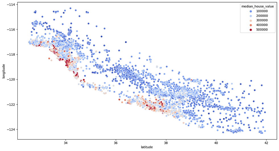
Reviewing the learned regression coefficients sheds light on which factors drive home values. Median income typically has the largest positive weight, confirming its role as the strongest predictor. The ratio of bedrooms to total rooms often carries a slight negative weight—higher values imply smaller average room sizes, which tend to lower market value. Conversely, the number of rooms per household usually receives a positive coefficient, reflecting that more spacious homes command higher prices. Spatial features like the one‑hot ocean proximity categories may receive smaller but still meaningful weights, indicating premium effects of living near the coast.

Conclusions and Next Steps

Our simple linear model captures roughly sixty percent of the variability in California housing prices, with a typical prediction error on the order of tens of thousands of dollars. To boost performance, we can explore adding nonlinear transformations (such as quadratic terms or interaction effects), applying regularized regression (ridge or Lasso) to mitigate overfitting, or moving to tree‑based ensembles like random forests or gradient boosting that automatically capture complex patterns. Incorporating richer geospatial features—distance to employment centers or school quality metrics—can also yield further gains. Each of these extensions offers a clear path to refine our predictive model while deepening our understanding of the factors that shape real‑estate markets.